
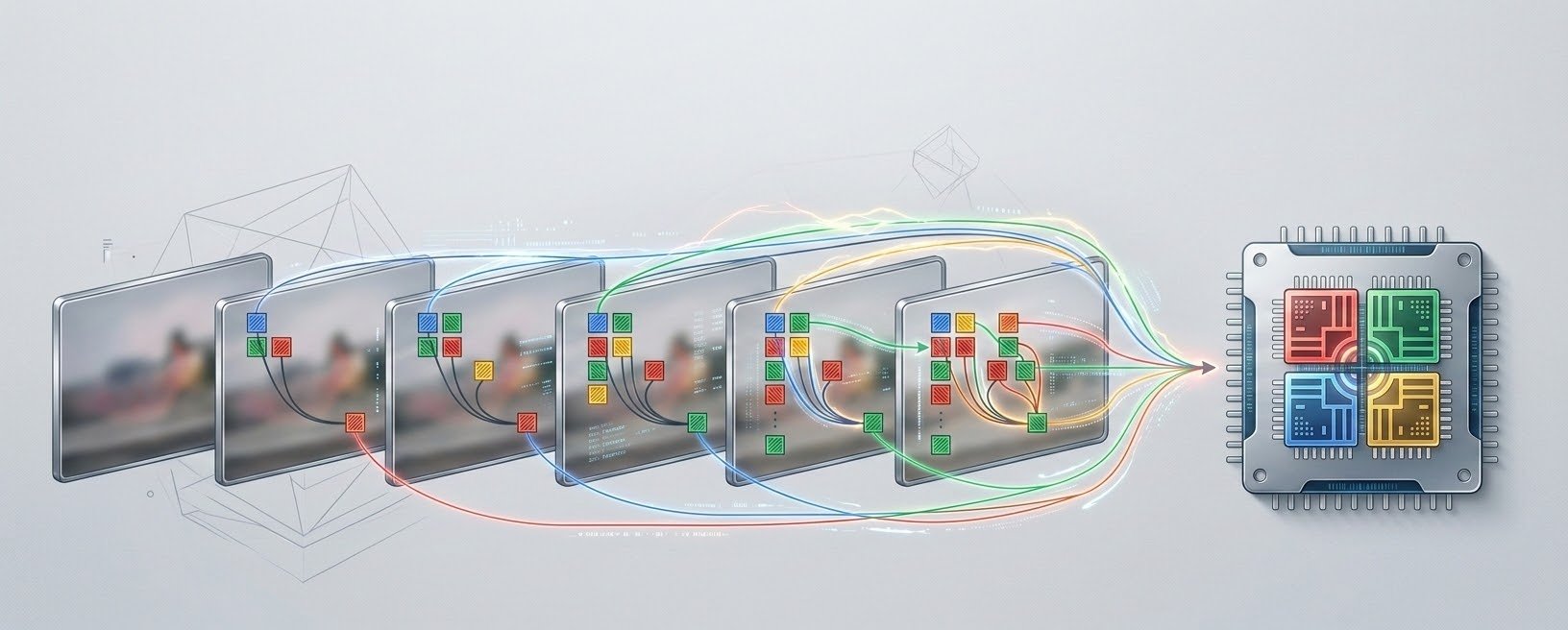
Video diffusion models are typically slow at generating videos for two reasons: a large number of denoising steps, and high cost for each individual denoising step. At large video sequence lengths, self-attention can become one of the dominant contributors to the latency of an individual denoising step. The sequence length for just 81 frames of 720p video ranges from 50K to 400K for popular open source video generation models today.
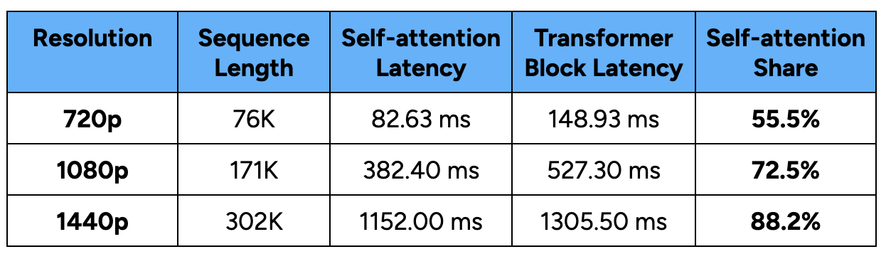
As an example, scaling from 720p (HD) to 1440p (2K) can quadruple the sequence length. Because full attention scales quadratically with sequence length, its share of per-layer latency can grow from 55.5% to 88.2%.
Since attention is the single greatest driver of latency within a single step, any aggressive inference optimization would need to target attention first. Fortunately, attention in video diffusion is highly structured: many query-key interactions carry little attention mass, so a large fraction of the pairwise computation can often be skipped. Dense attention computes every interaction regardless of its importance, while sparse attention uses a mask to retain only the most important interactions and discard the rest. An example of an attention matrix from a video diffusion model is shown below to illustrate how tightly concentrated attention mass can be.
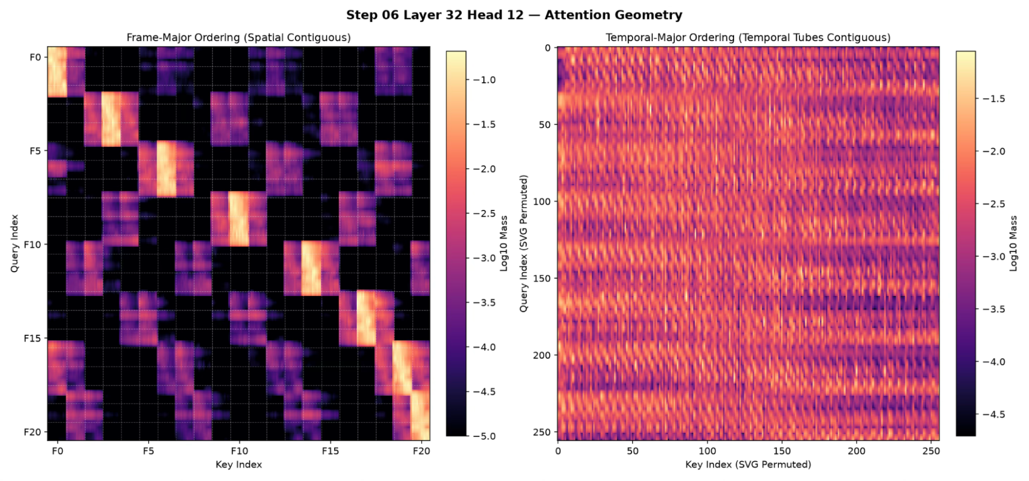
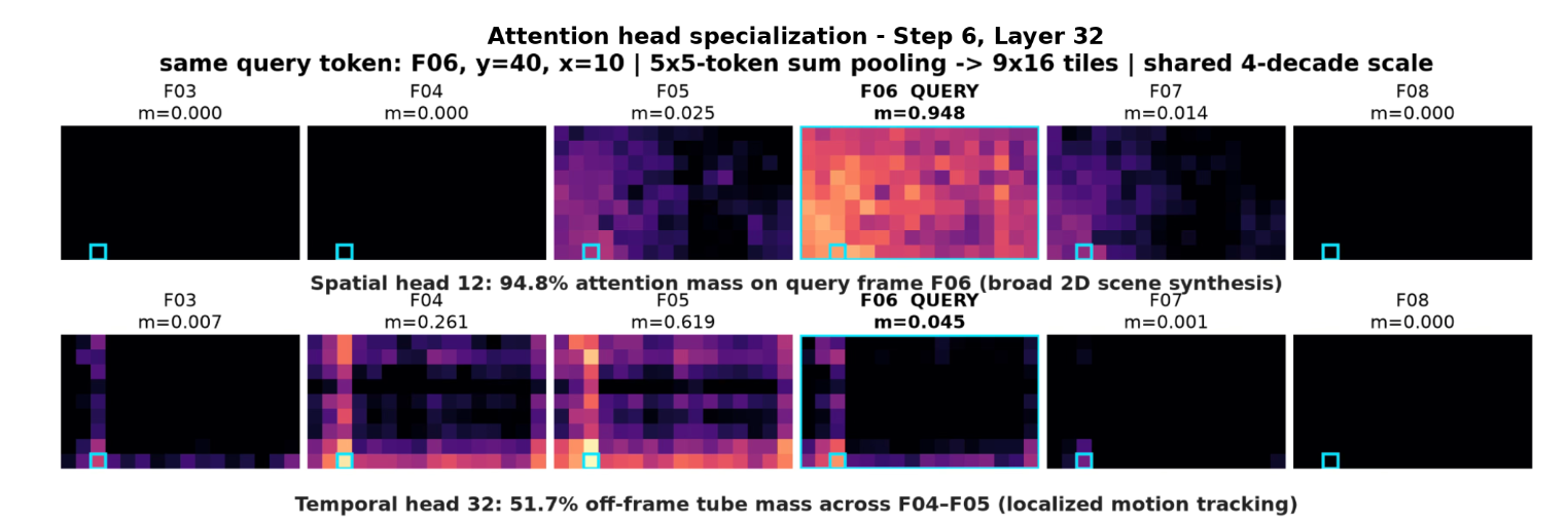
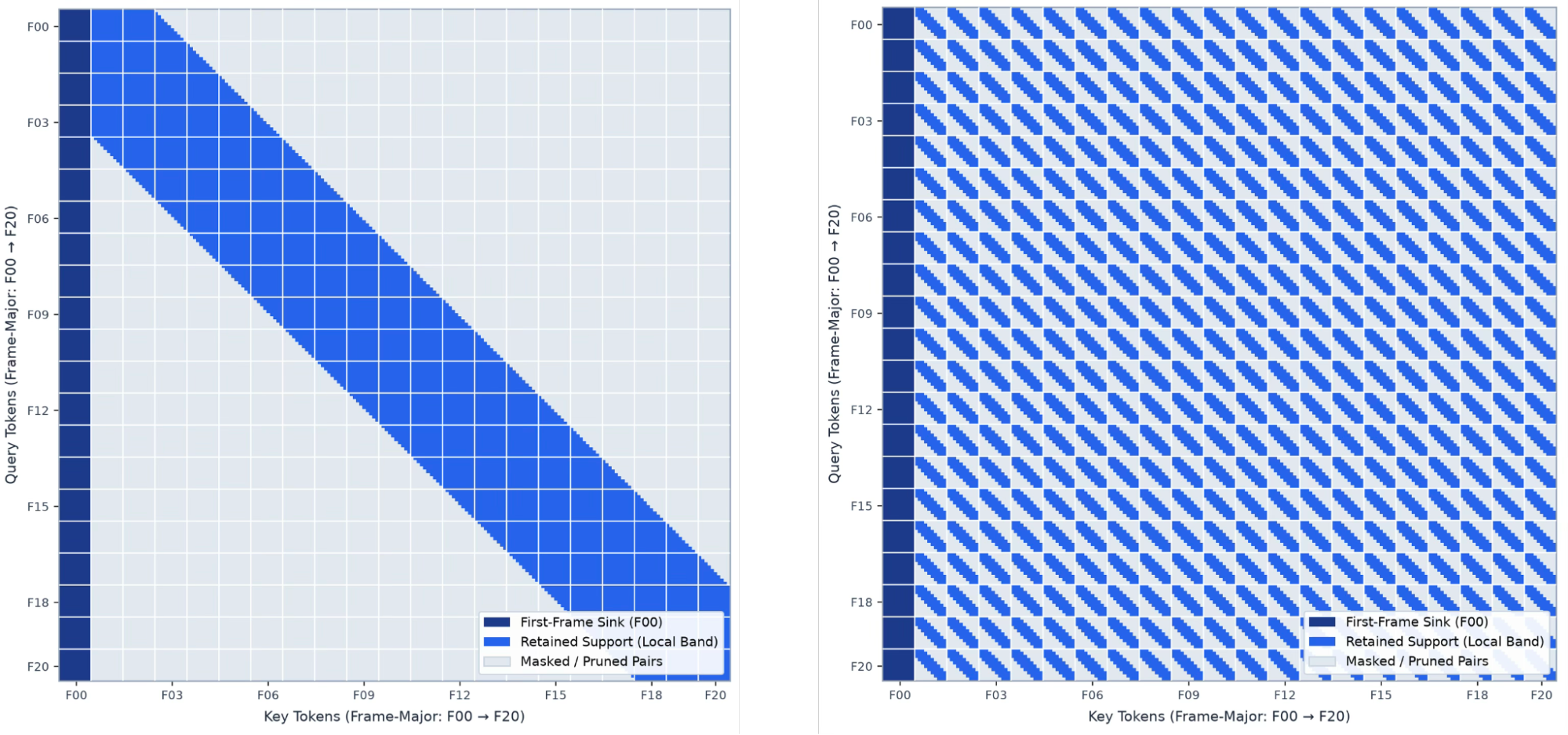
However, the pattern of attention varies across heads and layers, and even across steps. Sparse VideoGen (SVG) is a formative work that recognizes and exploits one pattern of attention: different heads are often characterizable as either spatial heads or temporal heads. Importantly for implementation, these are not arbitrary sparse patterns, and both have highly regular geometric structure. Within a spatial head, a patch attends mostly to other patches within the same or close-by frames; within a temporal head, a patch attends to a small spatial region across a large number of frames. In the image below, the attention mass corresponding to a single query is shown for a spatial head (first row) and a temporal head (second row). In the spatial head, the query diffusely attends to all the tokens in its own frame and to adjacent frames. In the temporal head, its attention is limited to a narrower spatial region but across a larger number of frames.
Based on this structure, SVG dynamically profiles attention heads at inference time and routes each head to either a spatial or temporal mask. It does so by sampling a small number of queries, computing their attention outputs under dense, spatial, and temporal attention, and selecting the sparse mask whose output deviates least from the dense baseline. This allows SVG to preserve higher quality at a given sparsity level. We refer readers to the SVG paper for details of the profiling and routing algorithm. As shown in Figure 3 below, both masks also retain full attention to the first frame (F00)—acting as an attention sink to anchor global scene appearance—alongside a local band for frame-to-frame interactions.
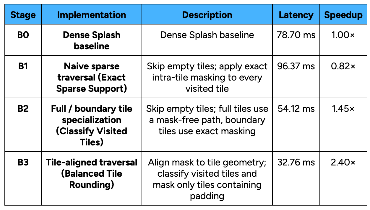
The table below summarizes the custom JAX and Pallas Splash Attention kernel implementations we compare. All timings use synthetic BF16 inputs on a single TPU v6e device, with 75.6K tokens, 10 heads, and a head dimension of 128. The reference query and key/value tile sizes are 3328 and 1536. Sparse variants retain approximately 38.87% of query-key pairs. These are isolated attention-kernel timings; routing, token permutation, and communication between devices are outside this measurement.
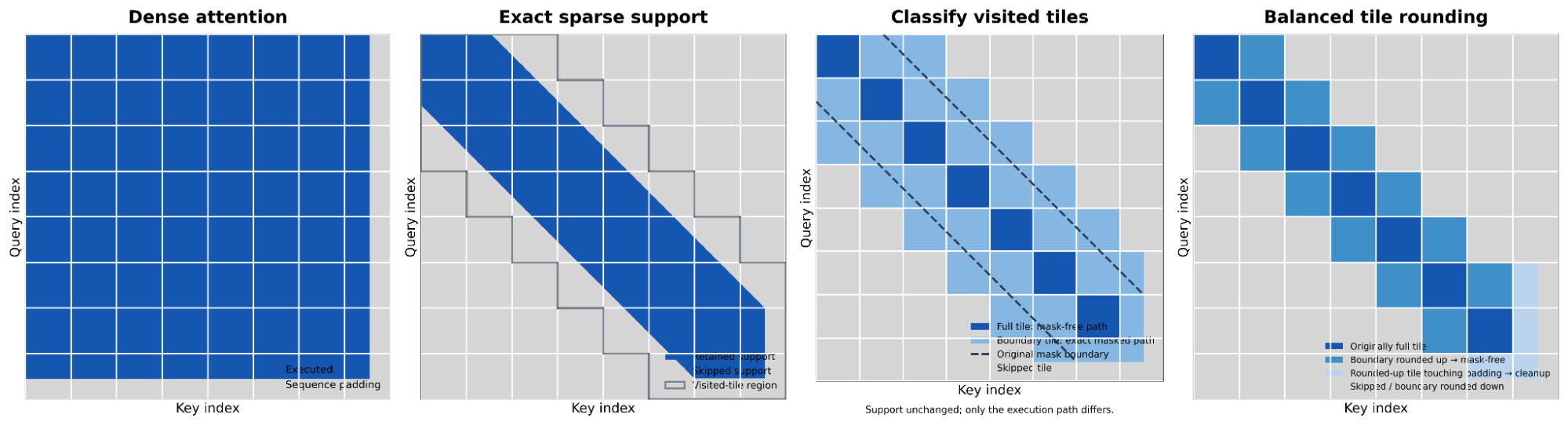
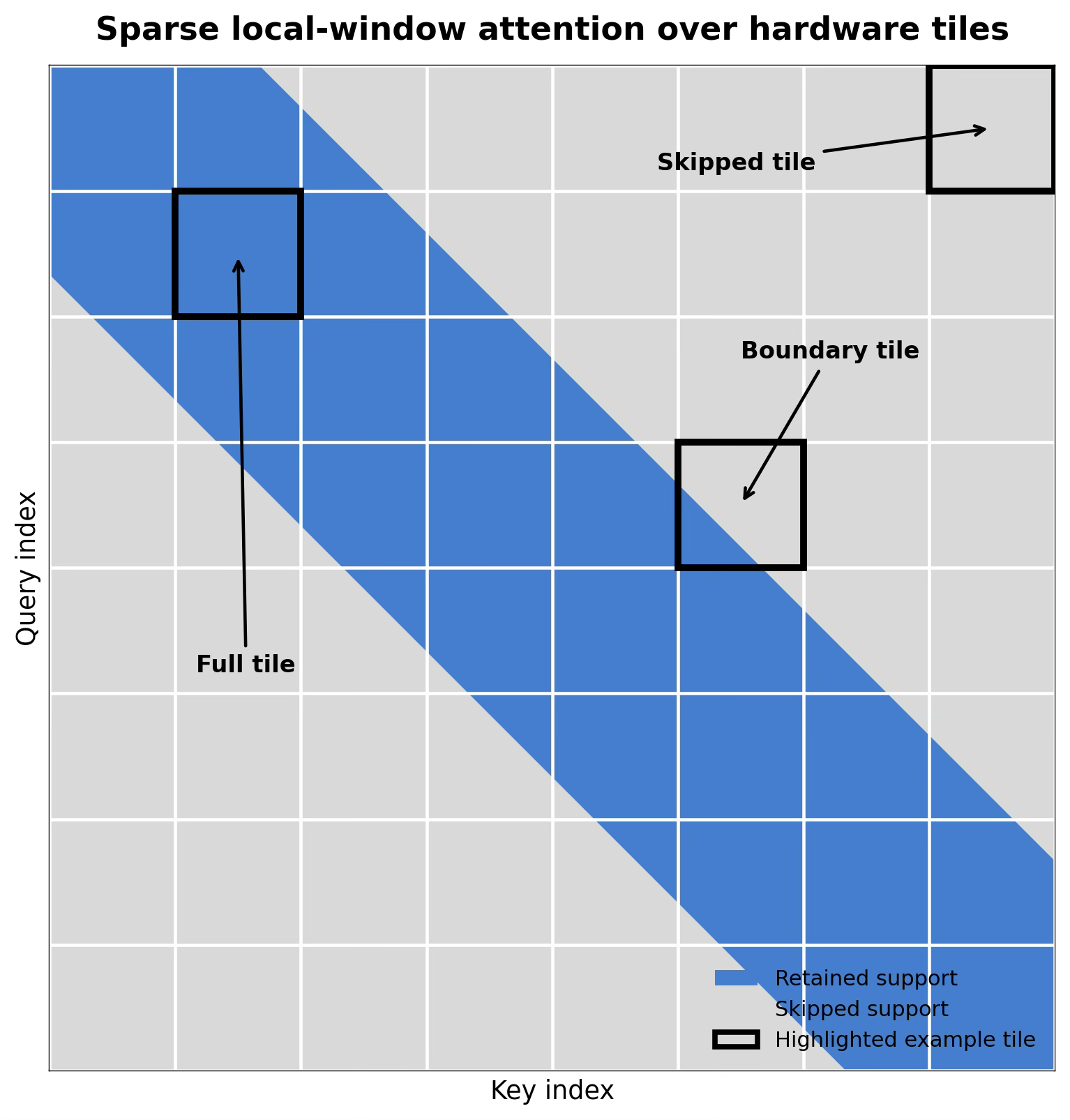
Although SVG has a clever approach to select an attention mask, this theoretical sparsity needs to be converted into a speedup on real hardware. Modern attention implementations don’t materialize the entire attention matrix multiplication Q · Kᵀ; rather, they divide it into tiles such as Q[i₁:i₂] · K[j₁:j₂]ᵀ and accumulate necessary statistics across these tiles to compute the attention output SoftMax(QKᵀ / √d)V. Within a visited tile, scores for excluded query-key pairs are set to negative infinity before the softmax so that they contribute zero attention weight. This enforces the mask, but does not avoid computing those scores in the first place.
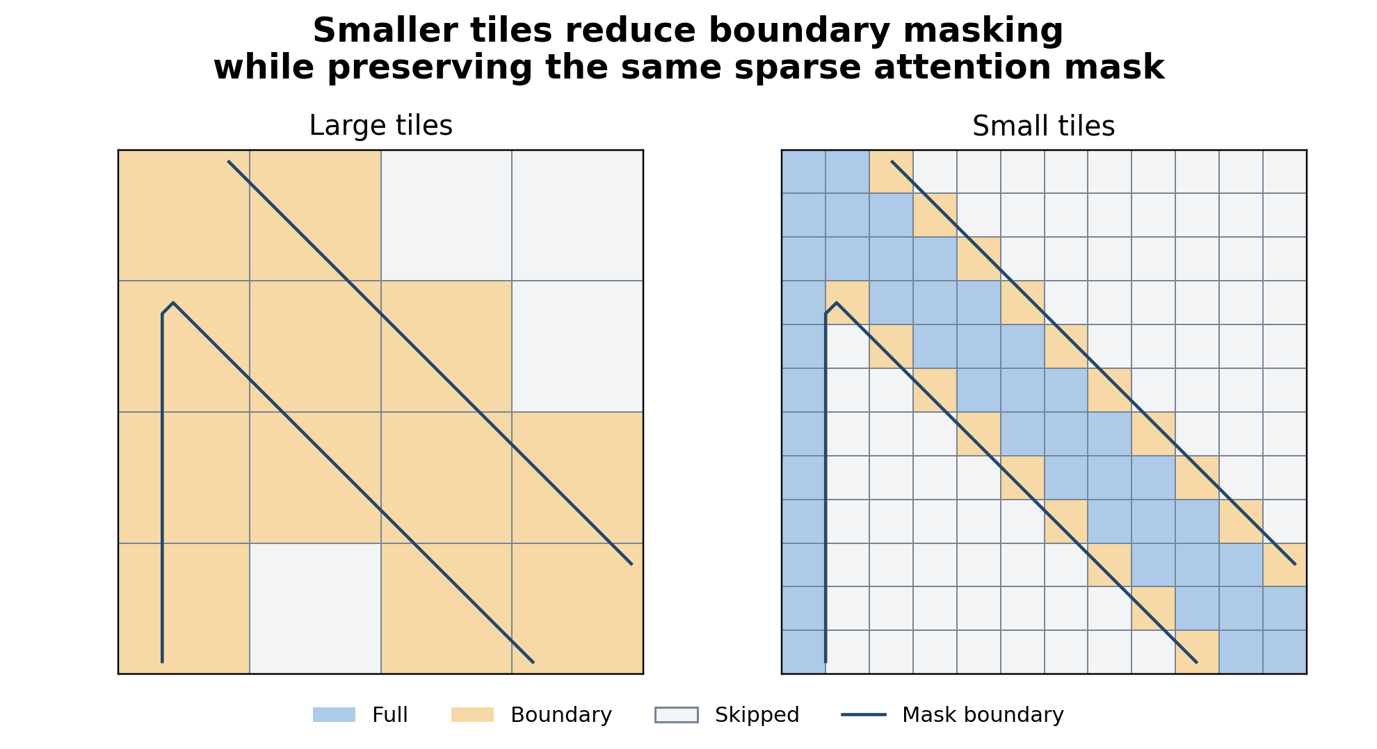
The mask divides tiles into three types. Full tiles contain only retained query-key pairs and need no intra-tile mask. Boundary tiles contain both retained and excluded pairs, so their scores need elementwise masking. Empty tiles (labeled Skipped tiles in the diagram) contain no retained pairs and can be skipped entirely. Logical sparsity counts excluded pairs, but the hardware savings depend on which tiles we can skip and how much work remains inside those we visit.
Splash attention already supports sparse masks and can skip empty tiles. However, this alone does not guarantee a speedup: how the kernel handles the tiles it visits also matters. In our initial sparse prototype (B1: naive block traversal), the mask retains 39% of query-key pairs, or about 61% logical sparsity. But the kernel visits 44% of outer tiles because boundary tiles also contain pairs that will be masked out. It skips the remaining tiles, but still evaluates the exact mask inside every visited tile. This implementation takes 96.37 ms compared to 78.70 ms for dense Splash: 22% higher latency despite skipping more than half the tiles.
Evaluating the exact mask requires determining which query-key coordinates are valid and applying that predicate to the attention scores. On TPUs, performing this elementwise mask evaluation on every visited tile bottlenecks the Vector Processing Unit (VPU) and stalls the Matrix Multiply Unit (MXU), even when every pair in a tile is valid. We can avoid that unnecessary work by identifying full and boundary tiles before executing attention and giving them separate paths.
To fix this, our second iteration (B2: full/boundary tile specialization) gives full tiles a completely mask-free fast path, executing exact coordinate masking only on boundary tiles. Both paths contribute to the same attention output, with their partial results combined using the corresponding softmax normalization statistics. The retained query-key pairs are unchanged. Latency drops from 96.37 ms down to 54.12 ms—a 44% reduction compared to the naive sparse traversal (B1) and 31% faster than dense Splash. This comparison shows the benefit of specializing tile execution while preserving the exact sparse mask.
Smaller tiles can follow the mask boundary more closely, reducing the fraction of tiles requiring intra-tile masking. However, tile size also changes how the kernel groups computation and data movement, so minimizing boundary work does not necessarily minimize latency.
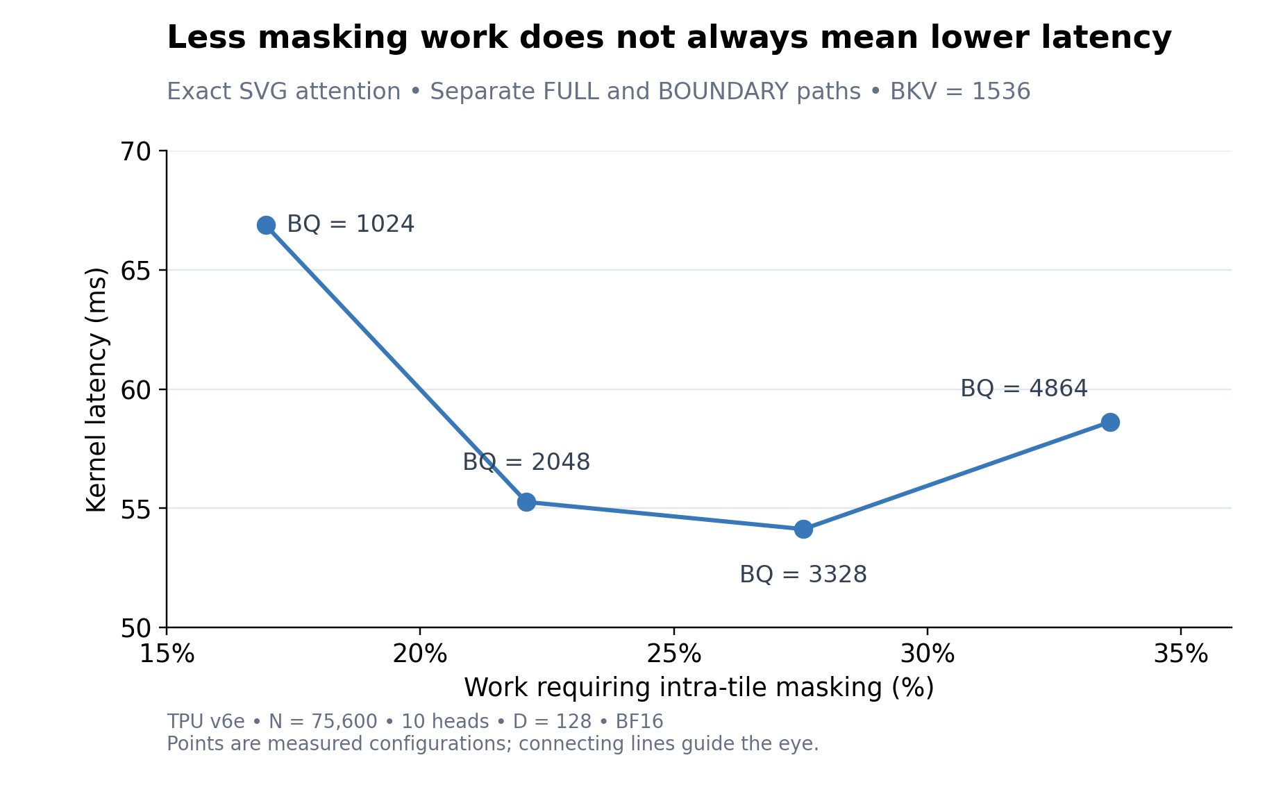
To illustrate this tradeoff, we vary the query tile size (BQ) while keeping the key/value tile size (BKV) fixed at 1536. Every configuration already uses separate full and boundary paths. At BQ = 1024, only 16.95% of executed tiles require internal masking, but latency is 66.88 ms. Increasing BQ to 3328 raises that fraction to 27.55% while reducing latency to 54.12 ms. Increasing BQ further to 4864 raises latency again, to 58.62 ms. The plot shows this tradeoff: the configuration with the least masking work is not the fastest. These percentages describe work/tiles requiring internal masking, not time spent evaluating the mask.
We can reduce boundary masking further by aligning the SVG mask with the tiles the kernel executes. Rounding a boundary outward includes some previously excluded pairs; rounding it inward removes some previously retained pairs. Balancing these choices slightly modifies the mask while approximately preserving the query-key pair budget. Unlike the previous optimization, this changes which interactions contribute to the output.
Rounding removes the need to enforce the exact SVG boundary within each visited tile. Because 75,600 tokens is not an exact multiple of the 3328 × 1536 tile dimensions, the edge tiles extending beyond the real sequence length still contain padding, and padded positions must contribute exactly zero attention weight. We therefore reuse the full/boundary distinction, with masking now needed only for tiles containing padding.
In our final configuration (B3: tile-aligned sparse traversal), this reduces the fraction of tiles requiring masking from 27.55% down to just 2.22%. Restricting masking strictly to boundary padding brings latency down to 32.76 ms—achieving a 2.40× speedup over dense Splash attention.
Together, these results show why sparse attention needs both a suitable mask and an efficient execution strategy: skip empty tiles, avoid masking full tiles, and align the overall mask with the tiles the hardware computes.
We now have a faster sparse attention kernel, but integrating it into distributed inference requires dealing with dynamic token layouts and different masks for different heads.
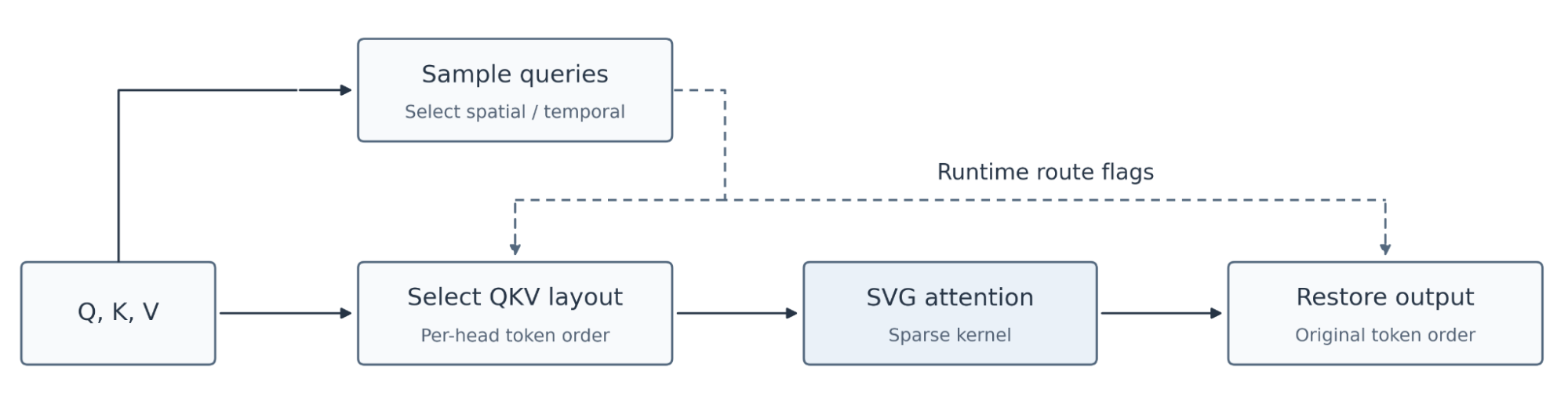
The routing step returns a Boolean flag for each head to select spatial or temporal attention. These flags choose between the original and permuted token layouts while keeping the tensor dimensions fixed. Unlike dynamically splitting heads into variable-sized spatial and temporal subsets, changing a head’s assignment at runtime does not alter tensor shapes or trigger costly XLA recompilations. The same flags restore temporal heads to the original token order after attention, so downstream layers receive the ordering that they expect. Spatial heads retain their original ordering.
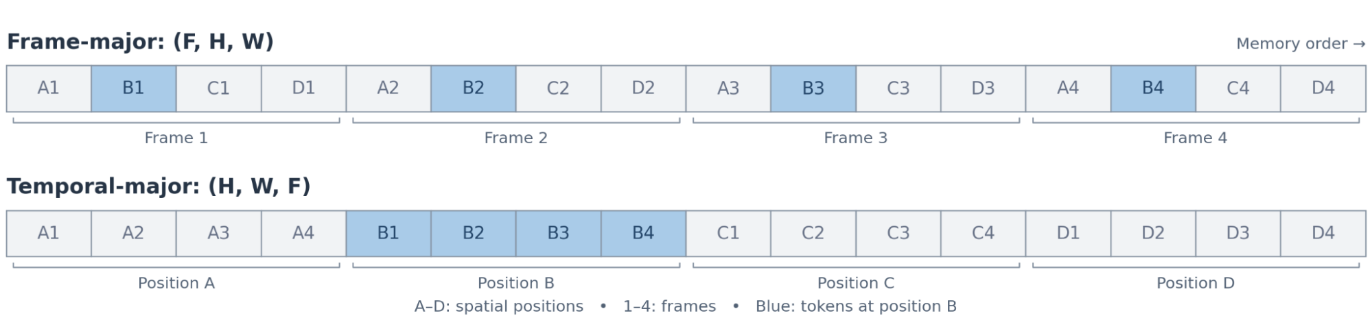
Permuting tokens from frame-major (F, H, W) to temporal order (H, W, F) places tokens at the same spatial position across frames next to each other—transforming the scattered diagonal stripes of the temporal mask (seen earlier in Figure 3, right) into a single contiguous band that the tiled sparse kernel can traverse efficiently. We tried avoiding this permutation and handling temporal access inside the kernel instead, but latency increased from 44.40 to 74.14 ms in our temporal-head benchmark, even though the faster path included additional overheads of permutation and restoration. This is in line with extra indexing and data rearrangement inside the kernel, although we did not measure those costs separately.
Where we perform this permutation matters in distributed inference. With 40 heads distributed across four devices, each device initially holds all 40 heads for one-quarter of the sequence. An all-to-all exchange redistributes this into 10 heads per device, each with the complete sequence. We call this the head-local layout.
Permuting tokens before that exchange can require additional communication because a head’s sequence is still spread across devices. After the exchange, every token needed to reorder a device’s local heads is already available there. We therefore apply the permutation after the input head exchange, execute sparse attention, and recover the original token order before the return exchange. Routing is computed before the exchange, and each head carries its routing flag with it.
In a matched TPU v6e experiment on one captured step and layer, moving token reordering into the head-local region reduced total attention latency from 75.64 ms to 46.81 ms, a 38% reduction. This includes routing, permutation, communication, and the sparse kernel. It shows why the placement of layout transformations matters alongside the sparse kernel itself.
Having optimized both the sparse kernel and its surrounding overheads, we now measure how these improvements translate into faster denoising. We evaluate 720p video generation with 81 frames, 40 denoising steps, and eight TPU v6e chips. The table compares three schedules that retain progressively fewer attention pairs, using the same prompt and seed and a local dense control for each configuration. Denoising times are medians of three warm runs, with speedup computed as dense time divided by SVG time. FFmpeg PSNR measures similarity between the encoded SVG and dense videos; higher values indicate closer outputs.
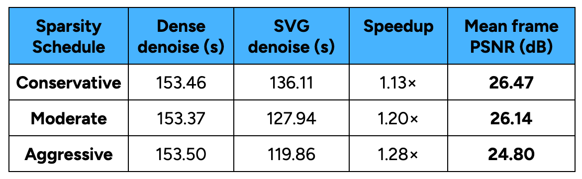
The aggressive schedule reduces denoising time from 153.50 s to 119.86 s, a 1.28× speedup and 22% lower latency. These results reflect the combined implementation with separately tuned dense and sparse configurations, including their distributed layouts. Gains are smaller than the isolated kernel speedups because denoising also includes work outside sparse attention.
Because self-attention accounts for an increasingly large share of transformer-block latency as sequence length grows—rising from 55.5% at 720p to 72.5% at 1080p and 88.2% at 1440p (2K)—end-to-end speedups from sparse attention scale substantially with resolution. Evaluating the aggressive schedule across resolutions shows how these savings compound on longer sequences:
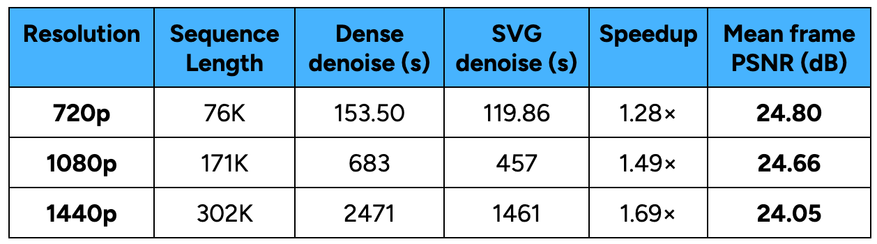
At 1080p (171K tokens), the aggressive schedule reduces denoising time from 683 s to 457 s (a 1.49× speedup at 24.66 dB PSNR). At 1440p (302K tokens, four times the sequence length of 720p), denoising time drops from 2,471 s to 1,461 s—achieving a 1.69× end-to-end speedup and saving over 16 minutes per generated video while maintaining 24.05 dB PSNR.
Key Takeaway: Efficient sparse attention on TPUs depends on how much work the hardware can avoid, not just how many attention pairs the mask removes. Skipping empty tiles, limiting intra-tile masking, and arranging tokens for efficient access helped us turn algorithmic sparsity into actual end-to-end generation speedups.

EmbeddingGemma 2: The Developer Guide

Integrating TorchTPU into TorchTitan and Optimizing Models for TPU

Bringing Visual Graph Debugging to Custom Edge Compilers with Model Explorer

Agent and Model Evaluations in Gemini Enterprise Agent Platform are now GA