
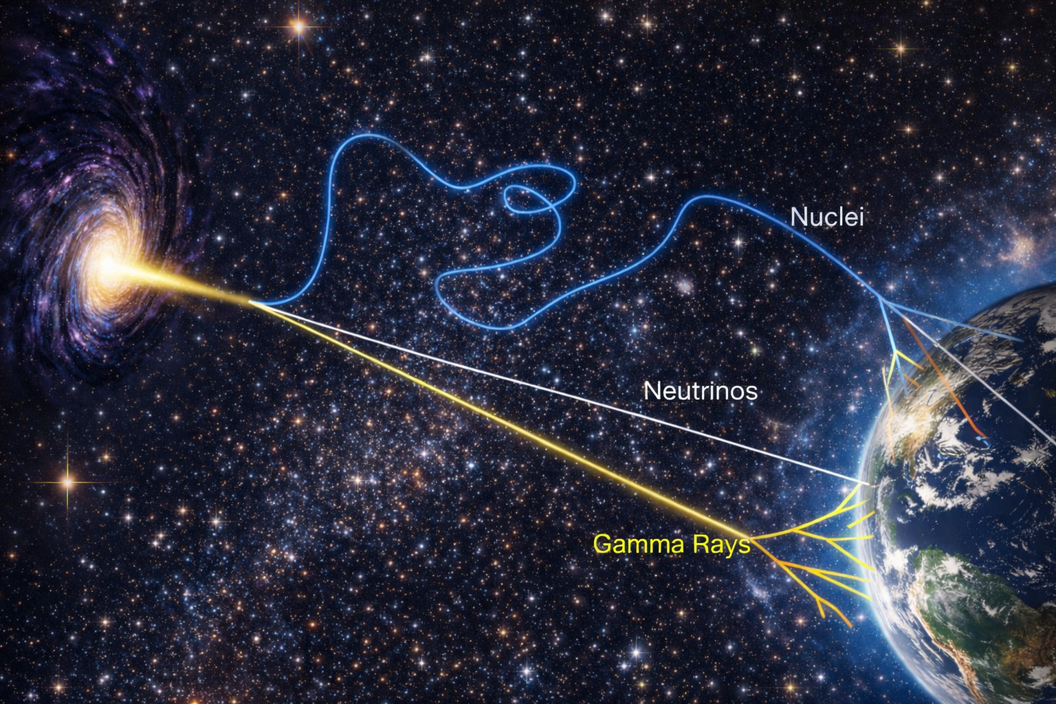
Astroparticle physics sits at the exciting intersection of astrophysics and particle physics and studies cosmic messengers: particles such as atomic nuclei, electrons, high-energy photons (light), and neutrinos accelerated in distant, cosmic phenomena and objects such as black holes, neutron stars, active galaxies, and supernovas, as well as other events from the early formation of the universe. By studying these messenger particles, we probe the most energetic and extreme phenomena known, from neutrinos produced in the Sun to the mysterious origins of ultra-high-energy cosmic-rays, and the elusive nature of dark matter and dark energy.
Modern astroparticle physics is inherently data-intensive. It relies on gigantic observatories, often spanning thousands of square kilometers, designed to detect rare and tiny signals from the cosmos. These instruments generate enormous volumes of complex data, far exceeding what traditional analysis techniques were designed to handle.
This blog post focuses on the growing role of deep learning in astroparticle physics and the new possibilities it unlocks in this data-rich research field. These methods offer new prospects to improve instrument sensitivity, uncover patterns that would otherwise remain hidden, and search for signal anomalies. Ultimately, these advances help to address some of the most fundamental questions: “What is the structure of the Universe?”, and “What is the elementary nature of matter?”
From stars and planets to galaxies and nebulae, astronomy is deeply rooted in the discovery and observation of fascinating objects in the Universe. In Astronomy, light (ranging from infrared to visible light, and all the way up to X-rays) is the messenger that is observed, providing the key to studying the cosmos. Astroparticle physics extends astronomy into the highest-energy regime, where the Universe reveals its most extreme phenomena. It looks at gamma rays (high-energetic photons, i.e., light), with charged nuclei, neutrinos, and most recently, gravitational waves. By observing not only a single messenger but combining multiple kinds, modern astroparticle physics opens a new window into the universe.
However, for observations at these high energies, quantum and particle-interaction effects fundamentally change how we observe the cosmos. Individual high-energy particles can no longer be detected directly at Earth using conventional observatories such as optical or radio telescopes. Instead, when the cosmic particles enter the atmosphere, they interact with air molecules and produce extensive particle showers — cascades of billions and billions of secondary shower particles, mostly electrons, positrons, muons, and light, that spread over large areas and reach the Earth’s Surface and extend over many square kilometers in scale. In fact, every second, about 100 of these secondary shower particles continuously pass through the human body, entirely unnoticed.
To make matters even more challenging, the flux of particles at the highest energies is extraordinarily low: at energies above 10¹⁹ electron volts, one expects only around 100 per square kilometer per century. As a consequence, astroparticle physics in the 21st century relies on enormous observatories, often covering tens to thousands of square kilometers, in order to collect sufficient statistics to perform surveys. These experiments enable physicists and astronomers to probe the Universe in ways that are inaccessible to traditional astronomy, astrophysics, and particle physics, opening a window onto the most energetic processes known in nature.
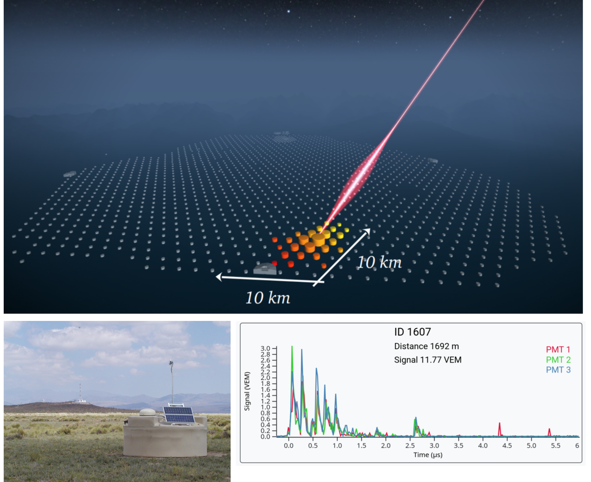
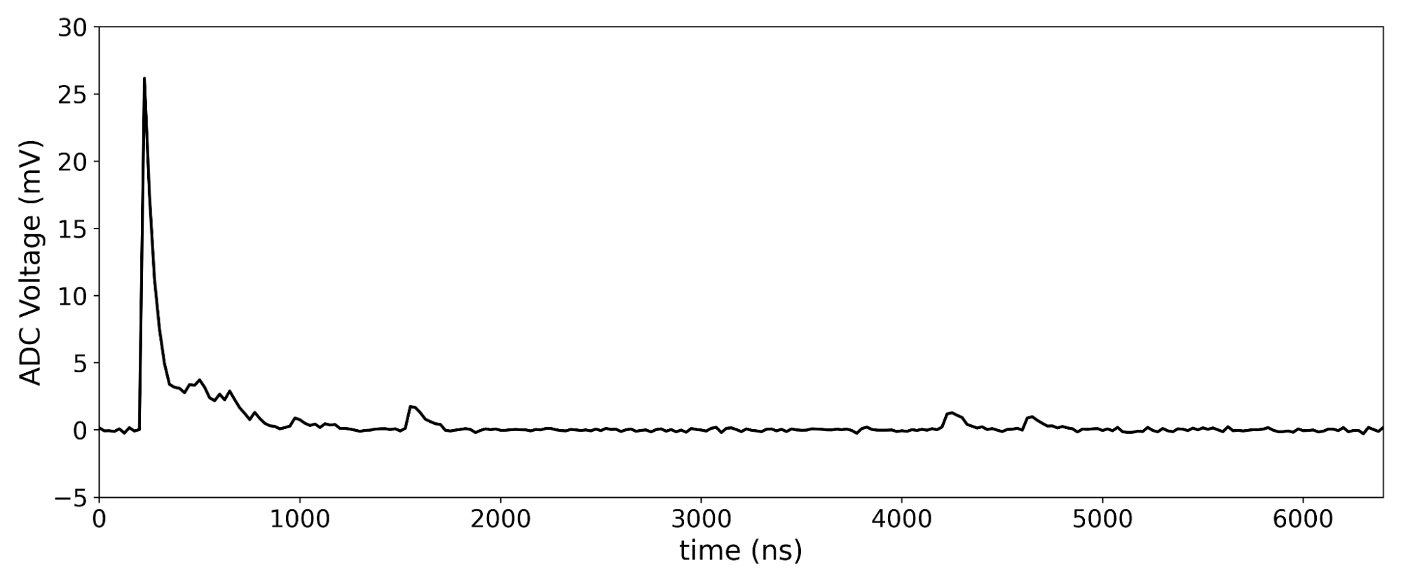
To catch the showers, sensors and detectors are distributed over vast, regular grids on kilometer scales or cubes, making their data image-like and well-suited for deep learning. Modern sensors usually feature readouts with nanosecond resolution that enable us to track the interaction of the incoming shower particles with the detector at high precision, by recording so-called waveforms or signal traces. An example is shown below for a cosmic-ray event measured by a detector of the Pierre Auger Observatory. As shown, different shower particles induce different shapes in the recorded total waveform.
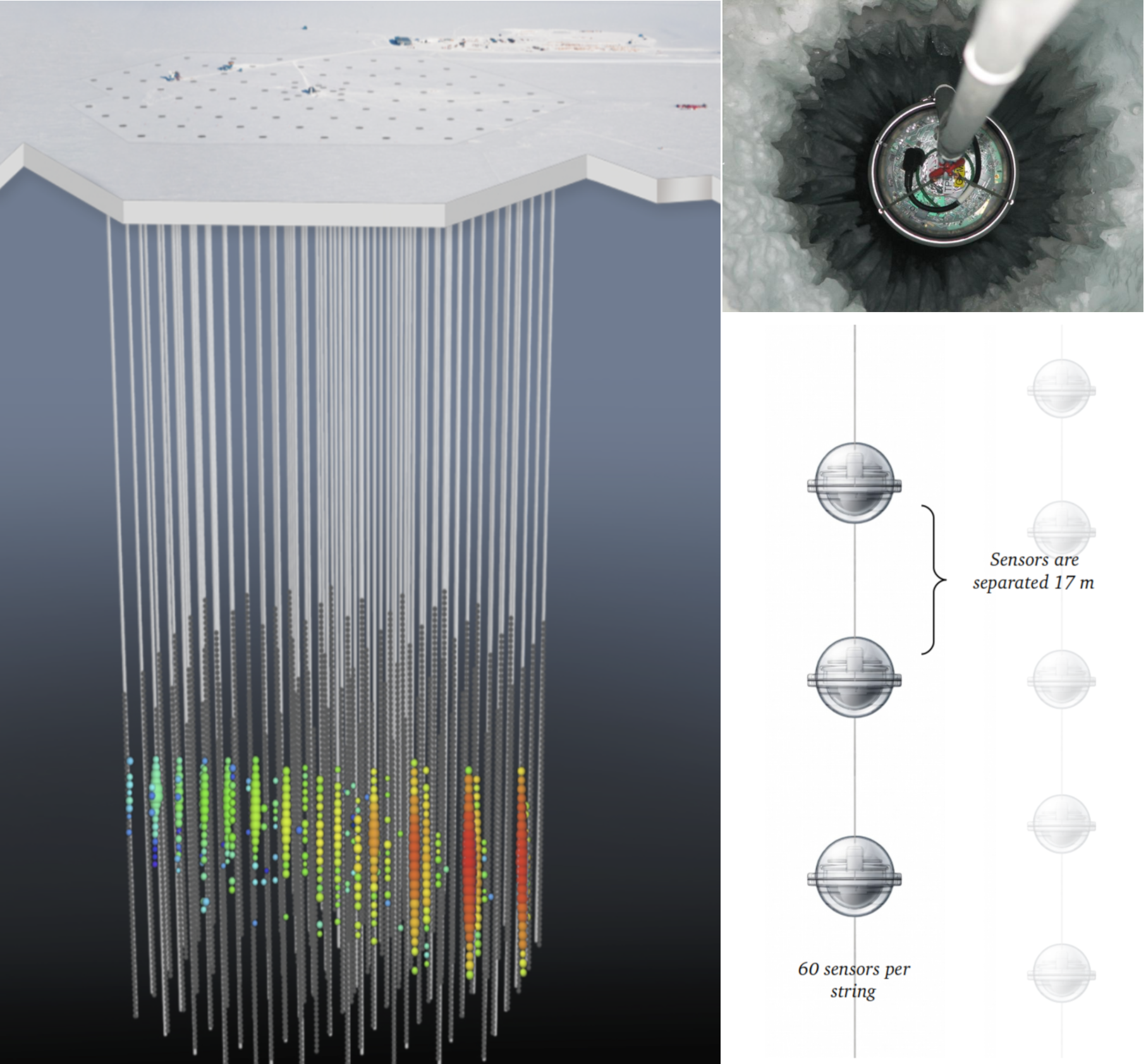
Prominent examples include the Pierre Auger Observatory, the world’s largest detector for cosmic-rays at ultra-high energies; the Cherenkov Telescope Array, the next-generation flagship facility for gamma-ray astronomy; and the IceCube Observatory, which uses a cubic kilometer of Antarctic ice to detect neutrinos (see the respective boxes). These observatories all have spatially distributed sensors that record waveforms, which encode information about the primary messenger particle, by providing spatiotemporal data structures of air showers.
The Pierre Auger Observatory, located in Argentina at an altitude of 1200 m is the world's largest cosmic-ray experiment and features more than 1500 detector stations covering an area of 3000 km^2. The experiment detects air showers at the highest energies, with each triggered detector recording up to three waveforms per event.
Neutrino telescopes such as IceCube in Antarctica or KM3NeT, currently under construction in the Mediterranean Sea, use strings of digital optical modules (DOMs) to detect faint flashes of light emitted by shower particles when they interact with ice or water. IceCube has an instrumented volume of approximately 1 km³ and is deployed as more than 80 strings, each equipped with 60 sensors, at depths between 1.5 km and 2.5 km beneath the Antarctic ice.
The Cherenkov Telescope Array Observatory (CTAO) is the next-generation facility for ground-based gamma-ray astronomy and is expected to collect more than hundreds of petabytes of data per year. It consists of two large arrays of Cherenkov telescopes. These telescopes are designed not to observe the incoming gamma rays directly, but instead image the Cherenkov emission produced by particle showers using ultra-fast cameras.
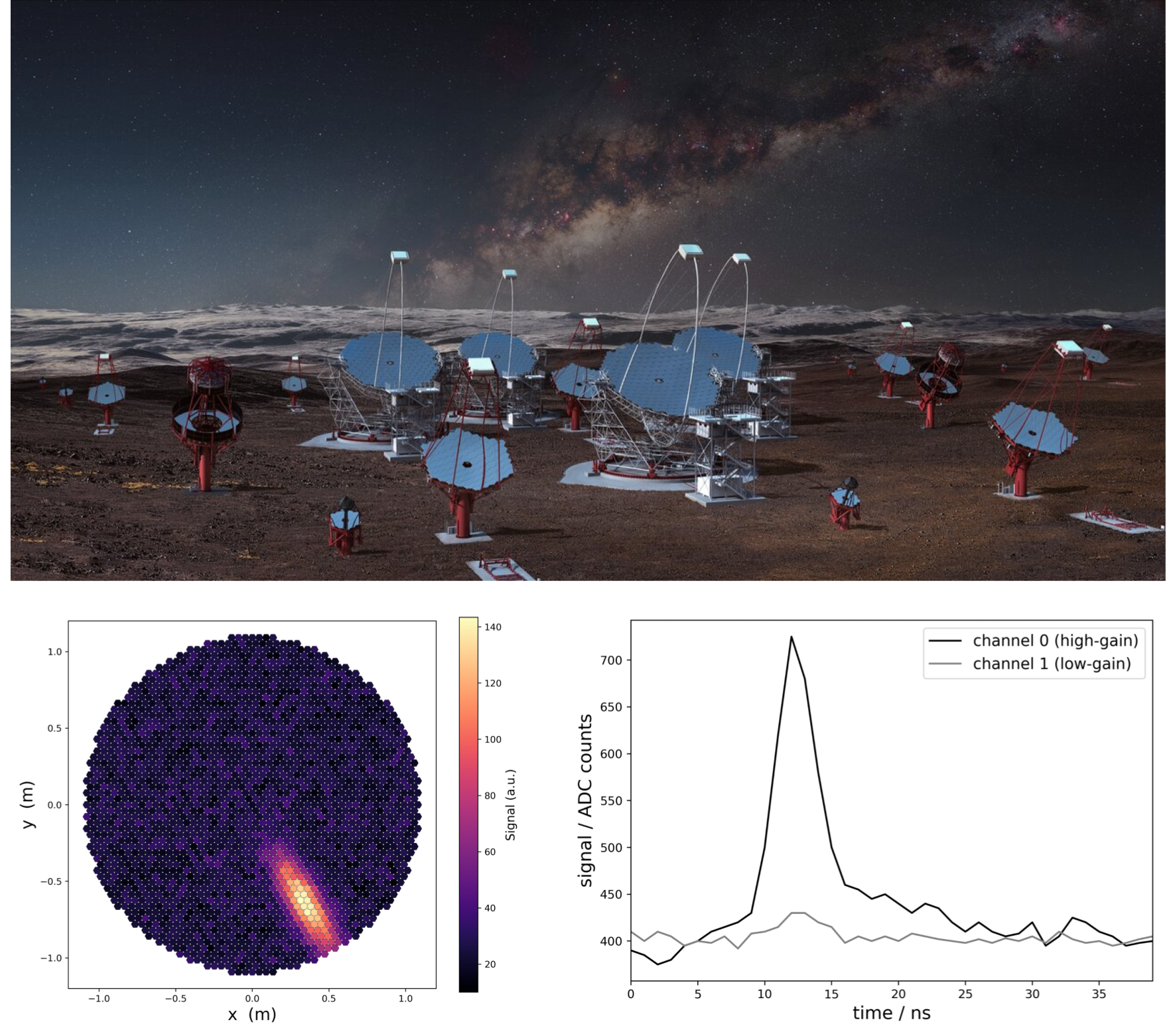
Reconstructing the properties of a cosmic particle from the measured shower data is exceptionally complex due to the indirect nature of ground-based detectors, as they don't catch the cosmic messenger directly. Instead, they sample the shower's footprint, i.e., the arrival times and energy deposits of particles hitting the ground. Figuratively speaking, the reconstruction is similar to a paleontologist studying bones to reconstruct the primary dinosaur. Similarly, with the signals recorded by detectors, researchers aim to infer the nature of the original particle (whether it was a neutrino, a gamma ray, or a cosmic-ray nucleus) as well as its energy and origin.
This reconstruction problem is particularly challenging because the development of particle showers is governed by stochastic quantum processes. Thus, each interaction underlies intrinsic fluctuations, meaning that no two showers are ever exactly alike, even if they were initiated by identical particles with the same properties (e.g., position and energy). As a result, precise and detailed measurements of the shower are crucial: the more information that can be exploited, the better the reconstruction of the primary particle — the messenger particle we want to study.
However, detailed measurements alone are not sufficient on their own. Interpreting these data requires highly sophisticated algorithms capable of identifying the underlying structures and patterns hidden within the shower signals and the huge amount of data. This formulates an inverse problem: from indirect and incomplete observations, the primary cause (cosmic messenger) will be reconstructed. This is precisely where deep learning comes into play. By learning complex, non-linear relationships directly from large volumes of data, modern methods offer powerful new tools to tackle the challenges of event reconstruction and enable more accurate and robust interpretations of astroparticle physics experiments.
Traditionally, event reconstruction has been performed via function fitting or using parametrizations derived from simulations or, where possible, first principles. These approaches rely not on the recorded waveforms themselves, but on two compressed quantities: the integrated signal, i.e., the charge, and the arrival time, defined as the time of the first particles hitting the respective detector. For reconstructing the energy E, usually a modified Nishimura-Kamata-Greisen (NKG) function:

is fitted to the integrated signal S of each station measured at a distance r to the shower center, with the remaining parameters either derived from shower simulations or optimized for the instrument. The result has a strong correlation with the primary energy and enables a reconstruction of good quality.
Reconstructing the mass of the primary particle is extremely challenging, as fluctuations in the shower development (the process that forms the cascade) often induce signal variations that are on the same scale or larger than the subtle differences induced by the tiny particles. Therefore, more phenomenological approaches have been introduced. A heavier nucleus — for example, an iron nucleus — fragments into many lower-energy sub-showers early in the atmosphere, creating a shower with a higher muon content relative to a shower induced by a lighter particle, e.g., a helium nucleus, of the same energy. These muons, which can be thought of as heavy electrons, travel nearly undeflected through the atmosphere and arrive at the surface in a sharp, narrow pulse, whereas other particles disperse over a broader time window. Traditionally, by quantifying the spikiness of the waveform traces using and comparing them to simulated air showers, the mass can be very roughly estimated.
Deep learning, and specifically Keras, offers a breakthrough, especially for replacing phenomenological approaches. Instead of relying on hand-designed features, deep neural networks can be trained end-to-end on simulated detector signals. The network learns to extract subtle, non-linear correlations between signal traces, their timing, and the detector geometry, reconstructing shower properties with unprecedented precision. This effectively bypasses the information loss inherent in reducing waveforms to just a single charge value and an arrival time, and enables the exploitation of the full spatio-temporal structure of the data — a fundamental limitation of current-generation reconstruction algorithms in astroparticle physics.
As an example, we will focus in this blog post on a neural network architecture developed by researchers at the Pierre Auger Observatory, based on Keras, to reconstruct the cosmic-ray mass composition from signals measured by its array of surface detectors. The architecture is tailored to the structure and symmetries of the data, as discussed in detail below.
The data recorded by astroparticle physics experiments and the Pierre Auger Observatory is spatio-temporal (see above: Pierre Auger Observatory), including sensors distributed in space that measure waveforms: each air shower imprints a pattern of particle signals across the detector array, evolving in both space and time. Its characteristic structure (e.g., signal size, shower particle composition, temporal structure) encodes information on the shower development, and thus the primary messenger particle. In particular, three physical aspects of the data are fundamental.
First, the measured shower footprint, i.e., the spatial distribution of the signals on the detectors. The footprint’s size directly correlates with the energy of the primary particle: a highly energetic cosmic-ray produces a shower so extensive that it triggers dozens of stations spread across many (tens of!) kilometers, whereas a lower-energy event leaves only a handful of stations with a small signal. Beyond its size, the shape of the footprint encodes the shower geometry. A circular footprint indicates a vertical shower arriving straight down, while an elongated and asymmetric footprint is induced by an inclined shower arriving from close to the horizon, where the shower front intersects the array at a shallow angle and travels across the array. In practice, only a small fraction of the 1,660 stations are triggered by any given event. To obtain a regular, image-like input suitable for convolutional processing, a 13×13 station cutout is extracted from the full array, with the station recording the largest signal placed at the center.
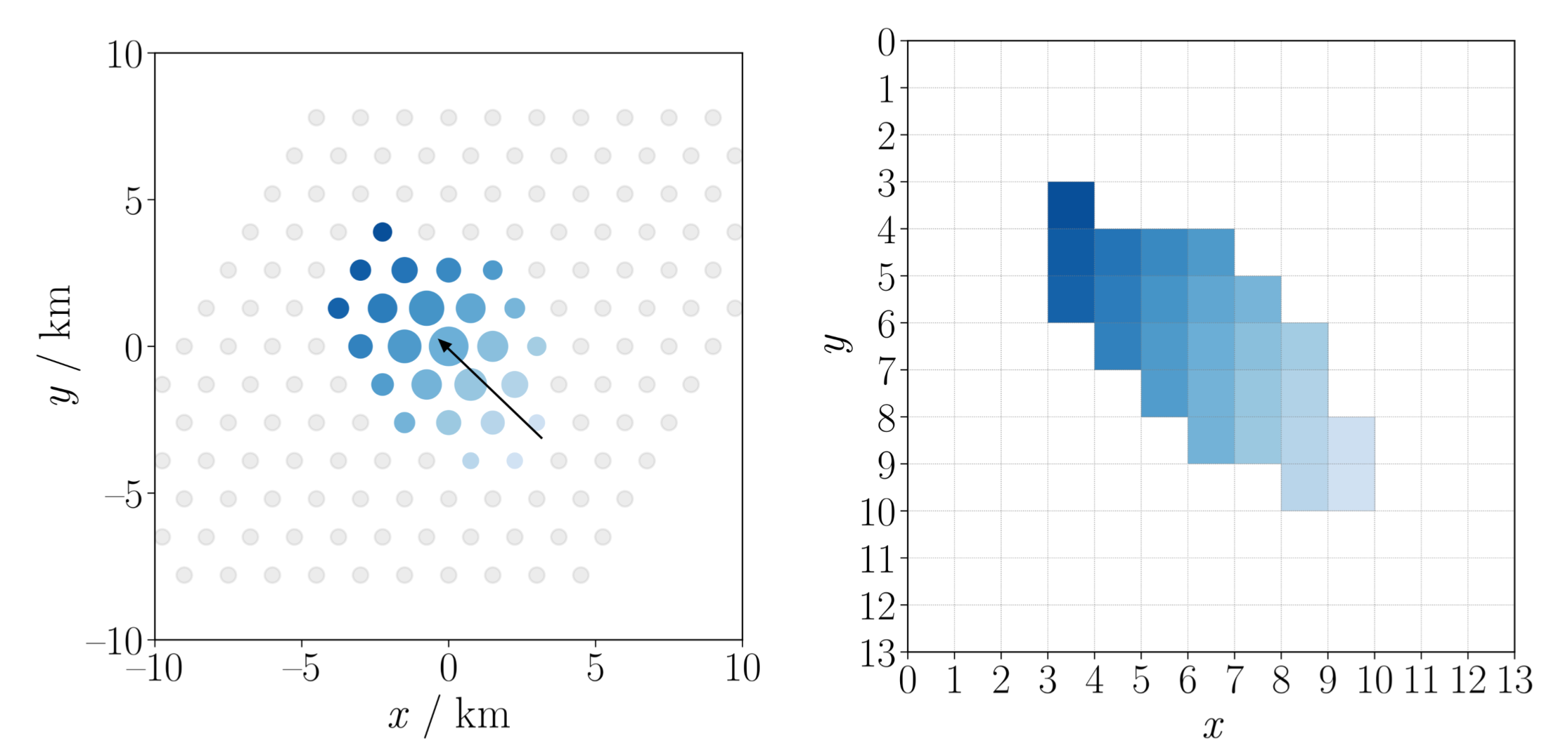
Furthermore, the arrival time, defined by the time the first particles arrive at each station — the leading edge of the waveform — encodes the curvature of the shower front as it sweeps across the array. These relative arrival times encode the shower’s direction and, therefore, also the direction of the impinging particle. Figuratively, this is similar to echo sounding, employing the arrival time of reflected sound to infer the depth and geometry of an object.
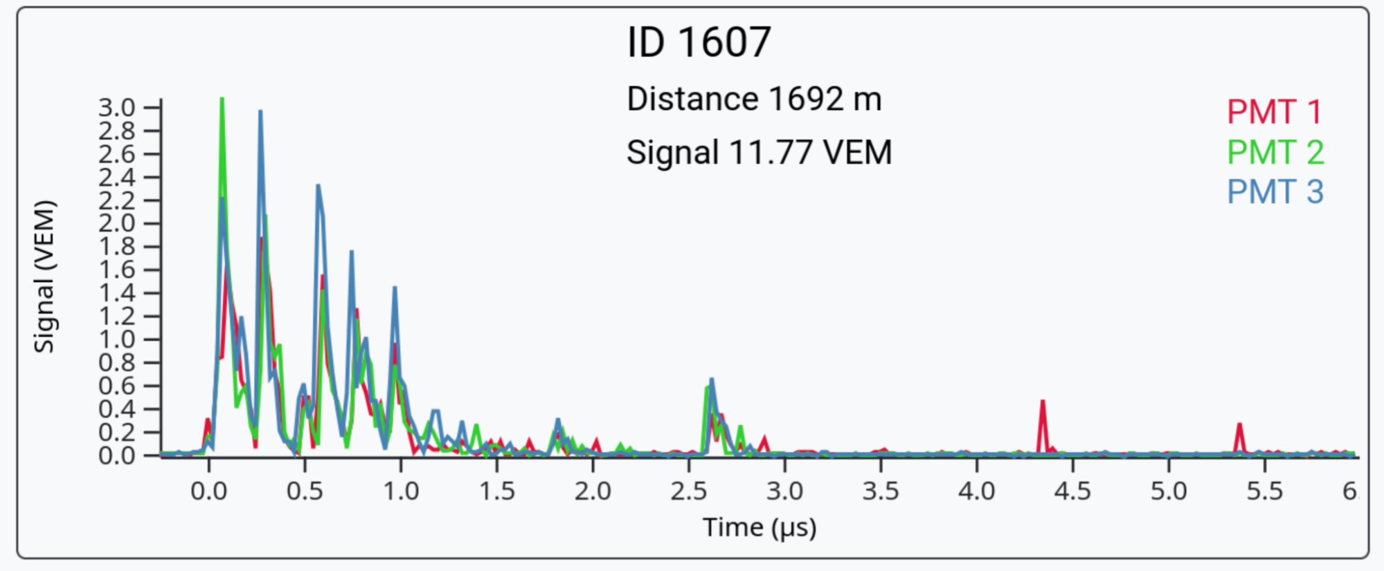
The shape of the waveform itself encodes information about shower development and mass composition. For example, showers with more muons will induce more spikes in the waveforms, whereas signals detected far from a shower that develops very high in the atmosphere will feature signals more spread in time due to the increased scattering of particles in the atmosphere. Auger utilizes 3 microseconds of the recorded waveform after an event is detected.
Using this cutout of the waveform instead of the full waveform (with only a short window containing meaningful signal) overcomes sparsity: instead of dealing with sparse traces, the network receives a scalar per station indicating when the shower arrived, along with three waveforms per station that encode information on the shower development.
Missing information is another key. In real-world observatories, detectors fail and stop working or fall close to the edge of the array where detectors are missing, causing missing information or holes in the footprint. It is important to note that it is fundamentally different from measuring having a signal data because a station is missing or broken, than a perfectly working detector does not measure a signal. To provide this information, a simple status map is added as input to the model (1=working, 0=missing/failing), and during training, detectors are masked and marked in the status map, respectively.
Together with the two-dimensional spatial layout of the stations, the full dataset forms a 3D data cube: a 2D grid of stations, each carrying a time trace of 120 steps, 25 nanoseconds each. A naive approach would feed this entire cube into a single big 3D CNN or similar architecture; however, this would not exploit the inherent physics symmetries, limiting the final performance as simulating air shower events is expensive and hence limited.
Instead, the setup is divided into two physically-motivated subparts: a temporal model that processes each station's waveform individually, and a spatial model that analyzes the spatial signal pattern induced on the detector grid. The key motivation is that, at a station spacing of 1.5 km, the waveforms at different detectors are causally independent — particles from the same shower arrive at each station separately, and there are no direct signal correlations between waveforms across stations. This means temporal and spatial processing can be cleanly decoupled, which is not only physically correct but also makes the model computationally very efficient.
import keras
from keras import layers


# =========================
# Temporal Model (LSTM part)
# =========================
class TemporalModel(keras.Model):
   def __init__(self):
       super().__init__()
       self.lstm1 = layers.TimeDistributed(
           layers.TimeDistributed(
               layers.Bidirectional(layers.LSTM(30, return_sequences=True))
           )
       )
       self.lstm2 = layers.TimeDistributed(
           layers.TimeDistributed(layers.LSTM(10, return_sequences=False))
       )


   def call(self, x):
       x = self.lstm1(x)
       x = self.lstm2(x)
return xThe temporal model processes each station's waveform independently. It applies a shared bidirectional LSTM followed by a standard LSTM to each of the three waveforms per station: the bidirectional LSTM scans all 120 time steps in both directions, and the subsequent LSTM compresses this into a vector of 10 learned features — a compact, learned representation of the temporal structure of that station's signal. These 10 features capture information that would traditionally require hand-engineering: things like rise time, pulse width, and muon-to-EM ratio, but learned from data in a task-optimized way. Using bidirectional LSTMs showed slightly improved performance over unidirectional (vanilla) LSTMs and makes it unnecessary to flip the trace, since most information is concentrated at the beginning of the time trace.
Critically, the same LSTM sub-network is shared across all 13×13 stations, enforcing that the physics learned from one station applies universally to all. This is a strong and well-motivated inductive bias: shower physics, as well as the interactions inside the detector, are universal, independent of where on the grid a station is located. In Keras, this weight sharing is elegantly achieved using the TimeDistributed layer, which applies the same Sequential LSTM layer to each station in the flattened grid, as seen at the top of the model definition above. Once each station has been reduced to its 10 temporal features, these are concatenated with the per-station arrival times and station status map onto the 13×13 spatial grid, and passed to the spatial model.
from keras.layers import Conv2D as ConvHex2D


# =========================
# SpatialModel: DenseNet-like
# =========================
class SpatialModel(keras.Model):
   def __init__(self, n_layers=3, n_filters=32):
       super().__init__()
       self.n_layers = n_layers
       self.convs = []


       for _ in range(n_layers):
           self.convs.append(
               ConvHex2D(n_filters, (3, 3), padding="same", activation="elu")
           )


   def call(self, x):
       dense_inputs = [x]


       for conv in self.convs:
           concat = layers.concatenate(dense_inputs)
           out = conv(concat)
           dense_inputs.append(out)


return layers.concatenate(dense_inputs)The spatial model uses convolutional layers across the spatial grid, underscoring the need for the temporal model to be shared across stations to enable effective convolutions of the feature maps (otherwise, the feature space of the temporal model would be only weakly constrained). While standard square convolutional kernels could be employed at the Auger array, hexagonal convolutions are better suited to the hexagonal detector grid and the inherent rotational symmetry of air showers (the measured detector signal is invariant under rotations along the azimuth angle). Therefore, group-equivariant convolutions are designed for hexagonal grids that enforce both translational symmetry and 60-degree rotational symmetry. This means the same convolutional filters are shared not only across positions (as in any CNN) but also across six rotational orientations, resulting in a parameter-efficient model that explicitly accounts for the rotational invariance of air showers, reflecting a well-founded physical inductive bias. In the pseudocode below, Conv2D has been aliased as ConvHex2D for illustrative purposes. To learn more about hexagonal convolutions, see the TensorFlow fork https://github.com/jglombitza/hexaconv of the HexaConv library https://github.com/ehoogeboom/hexaconv.
# =========================
# Individual Task Model
# =========================
def residual_unit(inp, nfilter, bottleneck=False):
   x = inp


   if bottleneck:
       x = layers.Conv2D(nfilter, (1, 1), padding="same")(x)


   shortcut = x


   x = ConvHex2D(nfilter, (3, 3), padding="same")(x)
   x = layers.Activation("relu")(x)
   x = ConvHex2D(nfilter, (3, 3), padding="same")(x)


   x = layers.Add()([x, shortcut])
   return layers.Activation("relu")(x)


# =========================
# Multi-task tower
# =========================
class MultiTaskTower(keras.Model):
   def __init__(self, nfilter=108):
       super().__init__()
       self.nfilter = nfilter


   def call(self, x):
       x = residual_unit(x, self.nfilter)
       x = residual_unit(x, self.nfilter)
       x = layers.AveragePooling2D((2, 2))(x)
       x = residual_unit(x, 2 * self.nfilter, bottleneck=True)
       x = residual_unit(x, 2 * self.nfilter)
       x = layers.GlobalAveragePooling2D()(x)
return xEmploying the hexagonal convolutions, the spatial model uses a densely-connected block inspired by DenseNet, where each layer's output is concatenated with all previous feature maps. This promotes feature reuse, preserving the arrival time, a physically critical feature throughout the network, which has been shown to stabilize training. Finally, after spatial pooling and a series of residual blocks, the network branches into separate task-specific towers for the energy, the cosmic-ray mass, and the arrival direction. This multitask structure is well motivated: the target labels are closely related, and learning them jointly improved both generalization and training stability.
# =========================
# Inputs
# =========================
trace_input = keras.Input(shape=(13, 13, 120, 3), name="TraceInput")
time_input = keras.Input(shape=(13, 13, 1), name="TimeInput")
state_input = keras.Input(shape=(13, 13, 1), name="StateInput")


# =========================
# Forward Pass
# =========================
trace_encoder = TemporalModel()
dense_block = SpatialModel()  # spatial model shared along all tasks
tower = MultiTaskTower()  # individual towers for each task


processed_traces = trace_encoder(trace_input)


x = layers.concatenate([processed_traces, time_input, state_input])
x = dense_block(x)
X = tower(x)


energy_output = layers.Dense(1, name="energy")(x)
xmax_output = layers.Dense(1, name="xmax")(x)
shower_core_output = layers.Dense(3, name="shower_core")(x)
shower_direction_output = layers.Dense(3, name="shower_direction")(x)


# =========================
# Final Keras model
# =========================
full_model = keras.Model(
   inputs=[trace_input, time_input, state_input], outputs=[xmax_output, energy_output, shower_core_output, shower_direction_output]
)


print("Model Summary:")
full_model.summary()This multitask network, trained end-to-end with physics simulations, unlocked a dataset ten times larger than state-of-the-art telescope observations, achieved with a detector never designed to actually measure cosmic-ray composition, and reaching energies at which no such measurement had previously been possible. A comparable result using telescope observations would require roughly 100 years of continuous operations.
The results confirmed that cosmic-rays become progressively heavier at the highest energies, ruling out the long-held assumption that pure protons are the most energetic particles in our universe. On top of that, the measurement revealed a characteristic structure in how the composition evolves with energy: it shows distinct features that align with known structures in the cosmic-ray energy spectrum, raising new questions about where and how these extreme particles are accelerated across the universe.
Insights of this depth were widely anticipated only after the completion of the AugerPrime detector upgrade, making their early appearance remarkable and promising an exciting future of cosmic-ray detection that combines deep learning, Keras, and AugerPrime.
The success of deep learning applications is not limited to a single experiment. For example, at the IceCube Observatory, deep learning has similarly changed event reconstruction and selection, leading to the discovery of neutrinos coming from the galactic plane. Across many physics experiments standard reconstruction algorithms struggle with complex event geometries, forcing physics analyses and surveys to exclude a large fraction of these recorded data to preserve high quality. In contrast, deep learning can recover previously unusable events, allowing more observation data to be analyzed quickly and efficiently, enabling timely follow-up observations. In both experiments, the Pierre Auger Observatory and IceCube, the power of deep learning enabled a ten-fold increase in usable observation data. To put that in perspective: ten times more data from a detector that has been running for ten years is equivalent to operating that same detector for a century. This leap in effective statistics is comparable to what a major detector upgrade or an entirely new observatory would deliver, projects that typically cost between one and ten million USD. The emergence of deep learning in astroparticle physics has only just begun, and as more and more observatories adopt deep learning in their reconstruction pipelines, there is more to come. The detectors we already have may yet reveal phenomena we haven't even thought of looking for…
A persistent challenge is the mismatch between non-perfect physics simulations and real detector data, which has largely limited the performance of deep learning in physics to date. Models trained on simulations that do not perfectly reflect real detector conditions make domain adaptation and careful cross-validation of the algorithms with independent detectors essential. Therefore, dedicated calibrations of deep learning algorithms using separate detectors are essential and can be combined with domain adaptation techniques to bridge the gap between data and simulations. Equally important is the precise quantification of uncertainties; unlike in many industry applications, physicists need very exact uncertainty estimates to test hypotheses and assess the likelihood of a discovery, requiring detailed studies to quantify model uncertainties, in particular when there is a domain shift between simulations and data.
In the future, foundation models that can facilitate a range of tasks: such as event reconstruction, simulation and unfolding, pre-trained across multiple experiments hold much promise for multi-messenger astronomy, where signals from multiple messengers: cosmic-rays, neutrinos, and gravitational waves are combined to improve overall model performance, obtain a coherent picture, and open a new window to our universe at the highest energies. Deeply tied to this is the implementation of domain knowledge and inductive biases. Encoding such knowledge and physics symmetries into neural network architectures has proven crucial, often because simulated datasets in physics are far smaller than those in computer vision or NLP, as simulating a single shower at the highest energies can take up to a week on modern hardware. During the development of the Keras model discussed above, RNNs and CNNs were state-of-the-art. Today, graph neural networks or point cloud transformers would likely be better suited to handle rotational symmetry and the sparse, irregular footprints, while transformers would replace LSTMs to avoid their computationally expensive structure.
The community working in the intersection of AI and physics is increasingly confronted by Sutton's "Bitter Lesson”. Historically, efficient methods that employ massive computation have outperformed solutions based on human knowledge. Also in physics, where fundamental symmetries have been at its core for more than 100 years, in many cases, more training data and efficient scaling can outperform physics-inspired architectures. For a physicist, this success is not just bitter but also unexpected and confusing, suggesting that implementing domain knowledge may not be the final end, but rather an intermediate step and a sign of progress, perhaps making this a rather bittersweet lesson.
Finally, a persistent tension remains in how we define "doing science". We, humans, and our intelligence and capacities are cognitively and physiologically limited, driving our preference for "nice, simple-looking" equations. A machine-learned "black box" will solve complex questions with superior performance, but will likely trade physical insight and interpretation capabilities for that precision. In the end, we want algorithms that can discover as we do: discovering causal mechanisms, symmetries, and physics laws on their own, and not systems that, however powerful, optimize for predictive skill over what we have already observed. Doing science is simply different from machines trained to perform similar tasks, and this is not inherently bad; in fact, they are powerful tools. But it reminds us that our episteme is defined by the pursuit of understanding and not merely optimizing for predictive accuracy. This current and evident contradiction promises an even more exciting future for research at the intersection of AI and fundamental science.
To dive deeper, you can read the original results, published in JINST, and Physical Review Letters.
For those looking to apply these ideas in practice and learn more about fast prototyping of physics models in Keras, physics-specific tutorials, and a broader overview of the field, visit deeplearningphysics.org.
[1] Pierre Auger Collaboration, Auger Open Data Portal — schematic map of the Pierre Auger Observatory (1600 water-Cherenkov surface detectors and 24 fluorescence telescopes, Mendoza Province, Argentina). https://opendata.auger.org (accessed August 2026).
[2] Pierre Auger Collaboration, "Photos — Galleries," Pierre Auger Observatory,, released under CC BY‑SA 4.0 International License; usage subject to the Observatory's media guidelines. https://www.auger.org/component/content/article/93-photos?catid=82&Itemid=435 (accessed August 2026).
[3] Pierre Auger Collaboration, Auger Open Data — Event Display, reconstructed cosmic-ray air-shower event (ID 141316557800), interactive ground-array/FADC-trace/LDF/FD-profile viewer. https://opendata.auger.org/display.php?evsel=1&nbmin=20&evid=141316557800 (accessed August 2026).
[4] IceCube Collaboration/NSF, "Neutrino IC170922 in IceCube," artistic rendering of the neutrino event that triggered the September 2017 multimessenger detection of blazar TXS 0506+056, in: ECAP news article, "Breakthrough in Multimessenger Astrophysics," 12 July 2018. https://ecap.nat.fau.de/index.php/breakthrough-in-multimessenger-astrophysics/
[5] IceCube Collaboration, "Schematic view of a neutrino detected in IceCube," Detector Gallery, IceCube Neutrino Observatory, University of Wisconsin–Madison / NSF. https://icecube.wisc.edu/gallery/detector/
[6] G. Pérez Diaz (IAC) / M.-A. Besel (CTAO) / ESO / N. Risinger (skysurvey.org), "Proposed CTA Telescopes," artist's rendering of the ~99-telescope Cherenkov Telescope Array southern-hemisphere site at ESO's Paranal Observatory, released 26 Aug. 2020. https://www.eso.org/public/images/2020-cta-paranal-comp-8k-trans-cc/
[7] K. Kosack (CEA Paris-Saclay) et al., "Getting Started with ctapipe", ctapipe documentation (CTA Observatory). https://ctapipe.readthedocs.io/en/latest/auto_examples/tutorials/ctapipe_handson.html

Bring multimodal semantic search to the edge with EmbeddingGemma 2

Reproducing Olmo 3 7B Pre-training in MaxText: case study of large scale training on TPUs
EmbeddingGemma 2: The Developer Guide

Accelerating Spatio-Temporal Attention for Video Diffusion on TPUs